

1. Topic selection
The H3 base is already very strong on aesthetics and general quality (high-grade official data, CFG distilled), so a purely aesthetic LoRA struggles to add value — our first attempt (a lighting LoRA) ended as a negative result. One viable differentiation is physical dynamics, which the base is relatively weak at (though still strong enough compared with other open source models). Topic selection decides the outcome; verify the base model’s weakness with a handful of comparison generations before investing in data work.2. Data curation
H3 is strong. Most stock footage looks worse than what it generates, and metadata filters can’t tell (under 20% usable yield). So we built a data pipeline: a VLM watches the frames for coarse screening, a human GSB blind test makes the fine cut, and preprocessing (next section) lands the winners on H3’s serving grid.- VLM rubric: five-field JSON —
category_ok / spectacle / quality / watermark / mostly_static; total = `0.5spectacle + 0.3quality + 2category_ok - 4watermark- 3*mostly_static`. About 5.4 s/clip on 8 GPUs — the full pool screens overnight.
- The GSB blind test is the final quality gate: randomized sides per pair, opaque video URLs (untraceable even from devtools), source revealed after each vote. It answers one question — “is this clip actually better than what H3 generates itself?” — and only winners enter the training set. Of the 500 pairs, 198 went to the dataset, 187 to H3, and 115 were draws; a draw does not enter either, so only ~40% of screened candidates survive (splash 40% / smoke 41% / explosion 38%). On the pairs that were decided the dataset only just edges H3 out, 51%.
- Long clips yield up to two non-overlapping windows (one 10 s source = 2 training samples sharing a caption).
3. Preprocessing
Data must land exactly on H3’s serving grid (the encoder rejects anything off-grid):
One ffmpeg pass:
fps=24, scale=...:flags=lanczos, crop=1344:768, setsar=1, cut to 107 frames
(the SFT reader rejects clips with non-square pixels). The training manifest is a
jsonl, one line per sample:
metadata.video, the field
releases before target read.
The output of sections 2–3 is published as
rockdu/WISA-80K-Practical-Dynamics-254
(254 windows + train.jsonl, fully curated and already on the serving grid) — to train
on it you skip both sections and go straight to training below.
4. Training
miles-diffusion-sft).
The recipe defaults are exactly the validated optimum: lr 3e-5, weight decay 0.01,
LoRA rank 64 / alpha 128, rollout batch 32 (1 sample per GPU per optimizer step),
--fsdp-flow-shift visual=12,audio=3, --fsdp-supervised-streams visual,
--diffusion-guidance-scale 1.0 (H3 has no CFG), --sft-offload-encoder.
miles-diffusion started with RL and later grew to cover SFT. Read a rollout here as whatever
produces the next batch of training samples — RL generates them, SFT encodes them. Each batch is
then consumed by --num-steps-per-rollout 4 optimizer steps. Both fit the same loop, which is
why iter_N counts rollouts rather than steps.
Performance reference (8×H200, 254 windows):
End to end, the default 3 epochs (21 rollouts, 84 steps) take 66 min from a cold cache;
10 epochs (70 rollouts, 280 steps) take 2 h 50 min cold, 2 h 31 min on a warm one.
Training leaves DCP checkpoints only. Export the LoRA with one single command:
adapter_config.json sidecar; sgl-diffusion loads it
directly via --lora-path.
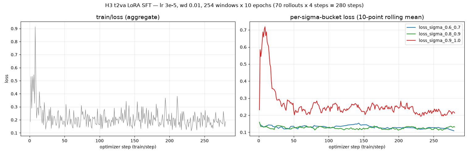
Reference loss (8×H200, same figure as the repo docs):
5. Training tips
Learning rate is extremely sensitive. Ablation on identical data and config (rank 64 / alpha 128, 254 windows × 10 epochs):
Other tips for DiT LoRA SFT:
- Watch bucketed loss, not the aggregate: DiT loss magnitude varies hugely with the
noise level, so the aggregate curve mostly reflects which sigmas a step happened to
draw — not training progress. The per-bucket curves from
--log-loss-sigma-bucket(default 10 buckets) compare like with like. - Quality beats quantity: ~200 clips that survived the GSB gate converge in 10 epochs and outperform larger, looser pools.
- Don’t train audio on noisy soundtracks: real-footage audio tracks are noisy, so the t2va
recipe passes
--fsdp-supervised-streams visual. The soundtrack is still encoded, noised and fed to the DiT as its native joint input, but excluded from the loss; drop the flag to train audio.
6. Results
Showcase
Known boundaries
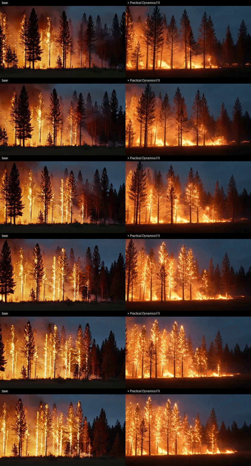
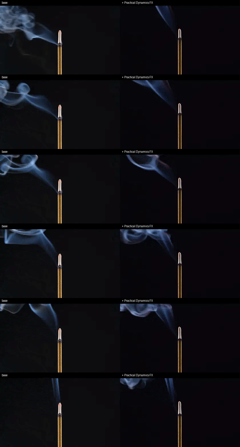
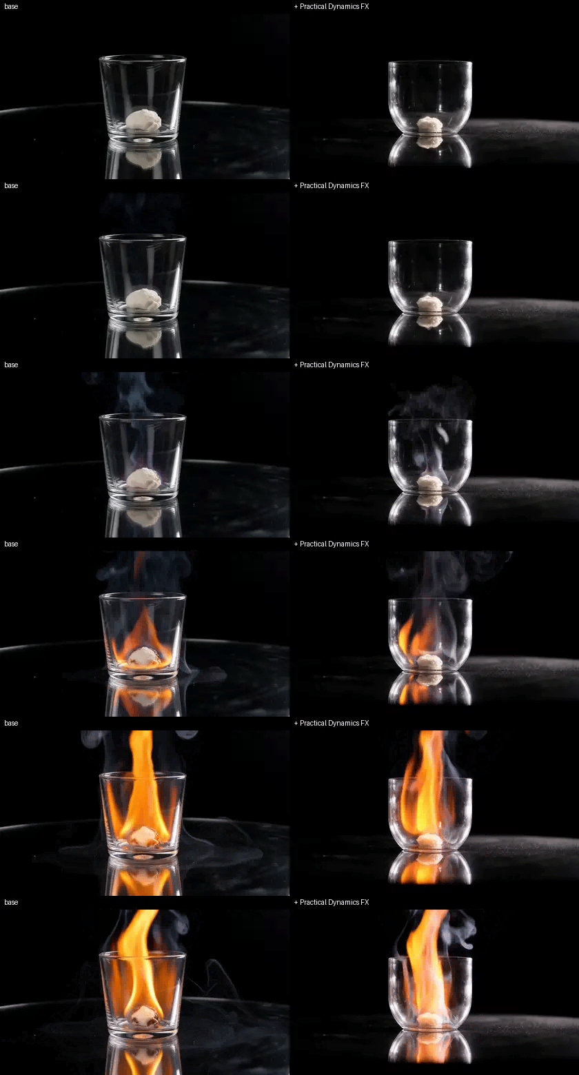
Generalization beyond the dataset’s distribution is limited. On ten out-of-distribution detailed prompts related to fire / explosions / smoke, the LoRA scored 6 wins / 3 losses / 1 tie against base — the reliable wins stay close to the training distribution.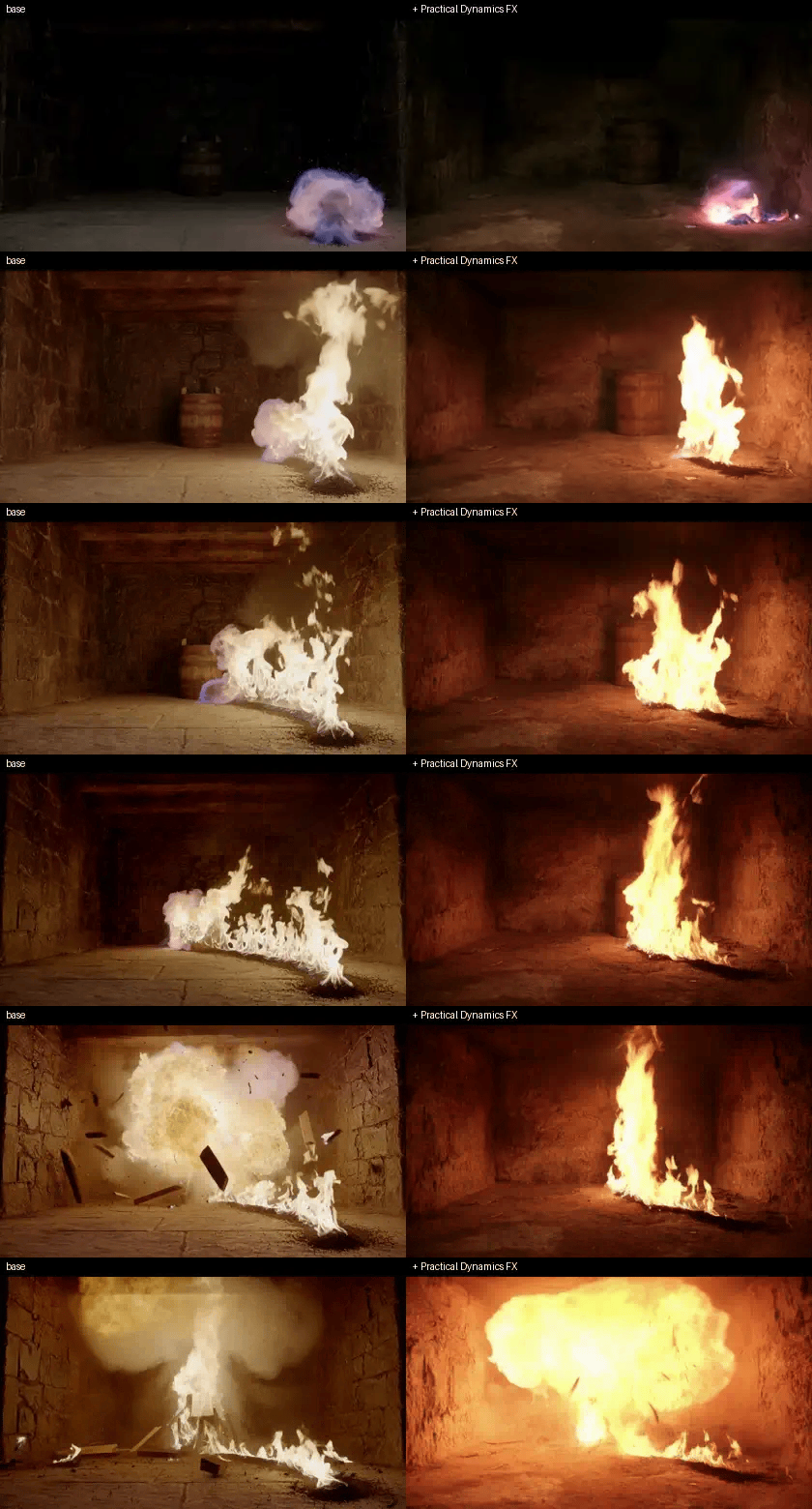
Artifact
practical_dynamics_fx.safetensors (rank 64, alpha 128, ~1.4 GB) + adapter_config.json.